1MASt3R on low-overlap drone imagery
Setup. A DJI flight on 14 August 2026 produced 36 photos; the 22 nadir frames were
used (four parallel lawnmower tracks, about 80 m above ground). Average forward overlap was only
~46%, which is below what classical SIFT/ORB pipelines like to see. The model was
the official naver/MASt3R_ViTLarge_BaseDecoder_512 checkpoint, run on
CPU only (AMD integrated graphics, no CUDA) at 512 x 288 px.
Experiment 1 — Can it reconstruct the scene at all?
Every candidate pair (sequential, jump, and cross-track neighbours within 60 m) produced at least 30 reciprocal matches. The strongest in-track pair gave 25,151 matches; cross-track pairs between parallel flight lines still gave over 20,000, which is what keeps the strips from drifting apart. The weakest were 85 m "jump" pairs at 60 to 121 matches — still valid. The estimated camera centres reproduced the four flight tracks. Output: a 50,000-point coloured PLY, 22 camera poses, and a diagnostic plot.
Takeaway. Dense transformer matching survives overlap that would break a keypoint pipeline. With a CUDA GPU the 21 minutes would be well under a minute.
Experiment 2 — Georeferencing with a 7-DoF similarity transform
MASt3R's scene is only relative. A Umeyama absolute-orientation fit (scale + rotation + translation) between the 22 estimated camera centres and the drone's onboard GNSS positions (local ENU) gave a scale of 73.83 m per model unit and:
Horizontal agreement is good. The vertical error is not noise: plotting the height residual against the along-strip coordinate shows a bowl-shaped (parabolic) drift, +5 m in the middle of the block and -7 m at the ends, with a fitted quadratic coefficient of 5.2 × 10⁻⁴ m-1. A rigid similarity transform cannot remove curvature; it comes from small pairwise tilt errors compounding along the strip when there are no ground control points.
Experiment 3 — Adding the barometer as a soft constraint
The drone's barometric relative altitude was remarkably steady (79.9 to 80.0 m AGL, about ±0.1 m precision) while its GNSS height is only ±2.5 m. So the trajectory was re-solved as a weighted non-linear least-squares problem with three terms: keep MASt3R's relative camera-to-camera vectors (weight 1.0), softly pull XY towards GNSS (0.5), and strongly pull Z towards the barometric flight level (10.0).
| Metric | 7-DoF similarity | Constrained solve | Change |
|---|---|---|---|
| Horizontal RMSE | 0.934 m | 0.786 m | -15.9% |
| Vertical RMSE | 3.593 m | 1.442 m | -59.9% |
| 3D RMSE | 3.712 m | 1.642 m | -55.8% |
| Max residual | 7.448 m | 3.212 m | -56.9% |
| Quadratic drift coefficient | 5.19 × 10⁻⁴ | 1.78 × 10⁻⁴ | -65.7% |
Some curvature remains because the visual term is kept stiff; flattening it completely would need non-rigid bending or, properly, ground control points.
1bOne photo, stereo, and fusing the two (September 2026)
Why. The MASt3R runs gave a coherent scene but metre-level heights. The next question was the cheapest possible input: can a single drone photo, with a recent monocular depth model (MoGe-3, released August 2026), give contours?
One photo. MoGe-3 on frame 12, scaled with the flight height from the photo metadata, compared with calibrated stereo from the two neighbouring frames. Shapes came out sharp, and on continuous open ground the error was 0.27 m RMSE — roughly a 1 m contour interval by the usual accuracy rule. But height differences between surfaces were wrong: the embankment stood 1.46 m above the swamp water in the three-photo stereo and 0.41 m in the single photo, and tree crowns came out far too low. Without correction, the raw output was bowl-shaped and tilted. Conclusion: one photo gives a sketch of shape, not elevations you can design with.
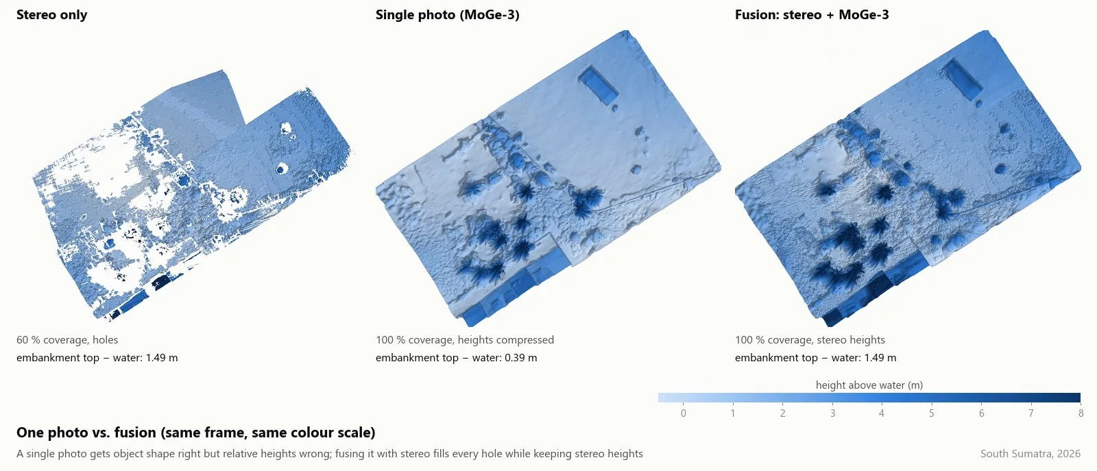
Fusion. Keep stereo wherever it exists; fill the gaps with MoGe-3 depth calibrated to the stereo around each gap.
| Hidden gap | Model alone | Stereo interpolation | Fusion | Fusion, open ground |
|---|---|---|---|---|
| 2 m | 0.80 m | 0.62 m | 0.20 m | 0.05 m |
| 6 m | 0.81 m | 0.96 m | 0.38 m | 0.08 m |
| 15 m | 0.64 m | 0.81 m | 0.45 m | 0.20 m |
The fused frame is 100% complete and keeps the stereo height of the embankment (1.49 m).
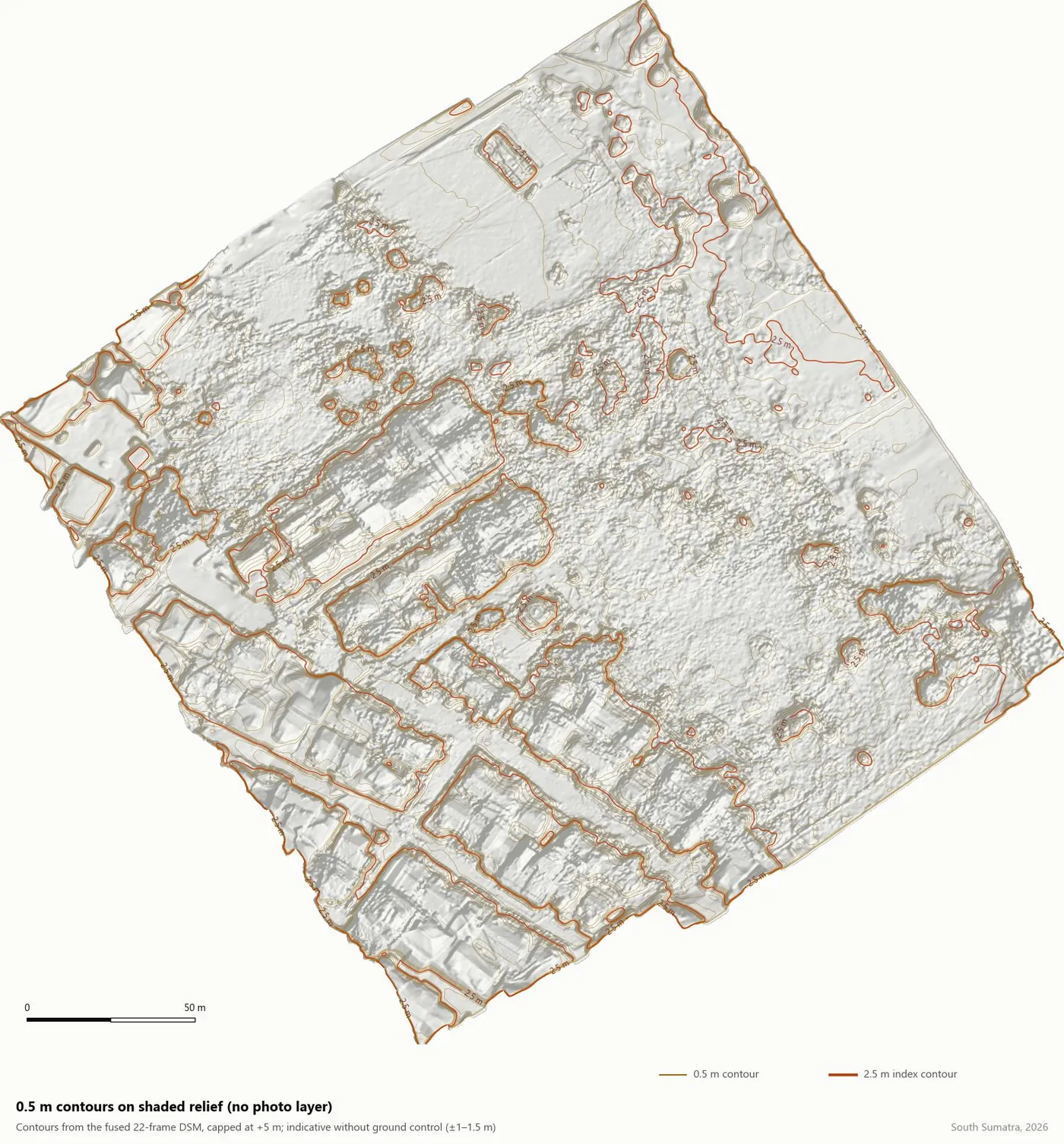
All 22 frames. Fusion was best in 22 of 22 frames for 2 m and 6 m gaps (median 0.25 m and 0.43 m). The mosaic covers 5.32 ha at 10 cm cells, 74% of cells from stereo, with 0.5 m contours. Aligning frames reduced the height bias between overlapping frames from 1.48 m to 0.17 m, but seams of about ±0.5 m remain.
2A low-cost integrated survey system (concept)
The problem. Irrigation and swamp-reclamation networks in South Sumatra run for thousands of kilometres. The standard survey (geodetic RTK, cross-sections every 50 m, manned echosounder, current meter; a crew of 4 to 6 covering 1.5 to 3 km a day) is accurate but so slow and costly that most of the network is never re-surveyed. Cost is linear in length, and the data is a sample, not a profile.
The idea. Four cheap, mostly open components chained so that each one's output feeds the next, written up in July 2026 as a discussion draft for a university research team, with the author as domain partner and field validator.
A. DIY RTK GNSS
Commercial GNSS module (LC29H / LG290P / ZED-F9P) + multi-band antenna, corrections from the national CORS network over NTRIP, an Android phone as controller. Centimetre positions for GCPs, checkpoints and the boat. Anti-false-fix procedure and raw logging for PPK as safety net.
B. Drone photogrammetry
Sub-250 g consumer drone with waypoint support, 100 m AGL, GSD about 2 cm, 80/70 overlap, processed in WebODM. Accuracy comes from GCPs measured with component A. Roughly 90 to 100 ha per day on three batteries.
C. USV bathymetry
Home-built catamaran (80 to 120 cm) carrying a 200 kHz single-beam echosounder and the RTK receiver, antenna mounted directly above the transducer so bed elevation = antenna height - offset — depth. Manual RC first, ArduRover autopilot later. Longitudinal runs give 15 to 20 km/day; zig-zag runs give cross-sections at 8 to 12 km/day.
D. Discharge by LSPIV
Drone video of the water surface processed with open LSPIV tools (RIVeR / KLT-IV) gives a surface velocity field; with the wetted area from C, Q = A x V. Cross-checked against a current meter and a Manning estimate from the RTK water-surface slope.
| Aspect | Conventional | Integrated system (design estimate) |
|---|---|---|
| Crew per day | 4 to 6 people | 2 people |
| Canal per day | 1.5 to 3 km | 8 to 12 km (with cross-sections), 15 to 20 km (profile only) |
| 100 km of canal | 40 to 60 crew-days | 8 to 12 crew-days |
| Equipment cost | Rental about Rp 1 to 2 million/day | One-off about Rp 25 to 45 million for the whole kit |
| Water-surface slope | Not available | Continuous, from RTK heights on the boat |
Rupiah figures are indicative and must be replaced with local unit prices; the structural point is that on a network of tens of thousands of hectares the saving is a multiple, not a percentage.
What makes it credible
Agencies judge the accountability of the numbers, not the brand of the instrument. The concept therefore treats validation as the core deliverable: every pilot segment surveyed both ways and compared statistically (horizontal, vertical, depth and discharge RMSE), independent checkpoints not used in processing, bar checks on the sounder, and documented LSPIV calibration. The roadmap is about 5 to 7 months part-time to a 5 to 10 km pilot, with validation piggy-backed on projects already running so the marginal cost is close to zero. Institutional route: a university research unit first, commercial survey contracts (which require certified firms and pilots) later.
How the two threads connect
The MASt3R experiments show what a consumer drone can deliver without ground control: a coherent scene with sub-metre horizontal but metre-level vertical error. Component A of the concept is the missing piece — cheap RTK-measured ground control points that turn that scene into something an engineer can sign. The next experiment is simply the same flight plus five GCPs.